Want to print the exported spreadsheet from the battalion line-up module of the DOC Log? The spreadsheet doesn’t work very well with default settings and so you’ll need to tweak a few things. Try this:

• Click the Page Layout tab at the top of the screen.
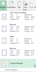
• Click on Margins (in the Page Setup section).  At the bottom of the menu that appears, choose Custom Margins.
  
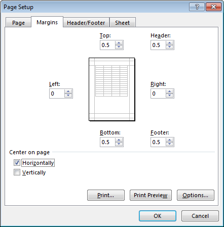
• Change the settings to:  Left: 0, Right: 0, Top: .5 and Bottom: .5
• In that same window, click Center on Page Horizontally.

  
  

• Click the OK button.
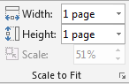
• While still in Page Layout tab, set Width to 1 page  and set Height to 1 page (in the Scale to Fit section).

  
  

• Click the View tab.
• Select Page Break Preview (toward the left side of the ribbon).  If a dialog box appears, click Do Not Show Again and then OK.
• You will see a blue margin line on the far right side of the document.  Drag that blue line to the left, all the way to the edge of the document where the blue shaded text box ends.
• Execute the Print command.

Note: To return to the previous view so that you do not see Page 1 written across the spreadsheet, select Normal, which is located next to Page Break Preview on the Page Layout tab.

Once you successfully print the first one, to print the additional battalions for your road pack, follow a similar process:

• Click the Page Layout tab and click Margins.
• Select Last Custom Setting (the first item in the list).
• Set Width to 1 page and Height each to 1 page while still in Page Layout, as you did earlier (above).
• Click the View tab and select Page Break Preview . You will see a blue margin line on the far right side of the document.  Drag that blue line to the left, all the way to the edge of the document where the blue shaded text box ends.
• Execute the Print command.